- Home
- SUMMARY
- BY TEXTBOOK Apri sottomenù
-
BY TOPIC
Apri sottomenù
- S1 : Greenhouse effect
- S2 : Anthropogenic cause
- S3 : Future scenarios of temperature increases
- S4 : Impacts on Earth’s systems
- S5 : Impacts on economic and social systems
- E1 : Mitigation as a social dilemma
- E2 : Carbon pricing
- E3 : Discounting in reference to climate change
- E4 : Inequality in reference to climate change
- E5 : Social Cost of Carbon and IAMs
- E6 : Persistency & irreversibility in reference to climate change
- E7 : Climate decision-making under uncertainty
- E8 : Climate policies
- E9 : Behavioural issues in reference to climate change
- E10 : Adaptation and geoengineering
- SAMPLE LECTURE
- ABOUT US
E6 : Persistency & irreversibility in reference to climate change
Any mention of the key terms persistence, delay, irreversibility or more generally stock externality linked with climate change will be recorded under this section.

US-5-m
694
GHG emissions do not cause the kind of immediate harm that sulfur dioxide emissions cause. Rather, it is the stock of accumulated GHGs in the atmosphere that ultimately causes harm. Furthermore, the dissipation rate for accumulated GHGs is very low: Once the GHG concentration in the atmosphere has increased substantially, it will remain high for many years, even if further GHG emissions were reduced to zero. That is why there is concern about reducing GHG emissions now rather than waiting for concentrations to build up (and temperatures to start rising) fifty or more years from now.
694-695
[In this section, 1, 2, t, t-1, N are originally in subscript in S1, S2, E1, E2, Et, St, St-1, SN]
Let’s focus on pollution to see how the stock of a pollutant changes over time. With ongoing emissions, the stock will accumulate, but some fraction of the stock, δ, will dissipate each year. Thus, assuming the stock starts at zero, in the first year, the stock of pollutant (S) will be just the amount of that year’s emissions (E):
S1 = E1.
In the second year, the stock of pollutant will equal the emissions that year plus the non-dissipated stock from the first year—
S2 = E2 + (1 – δ)S1
—and so on. In general, the stock in any year t is given by the emissions generated that year plus the non-dissipated stock from the previous year:
St = Et + ( 1 - δ )(St-1).
If emissions are at a constant annual rate E, then after N years, the stock of pollutant will be:
SN = E[1 + (1 - δ) + (1 − δ)^2 + ··· + (1 - δ)^(N-1)].
As N becomes infinitely large, the stock will approach the long-run equilibrium level E/ δ.
The impact of pollution results from the accumulating stock. Initially, when the stock is small, the economic impact is small; but the impact grows as the stock grows. With global warming, for example, higher temperatures result from higher concentrations of GHGs: thus, the concern that if GHG emissions continue at current rates, the atmospheric stock of GHGs will eventually become large enough to cause substantial temperature increases—which, in turn, could have adverse effects on weather patterns, agriculture, and living conditions. Depending on the cost of reducing GHG emissions and the future benefits of averting these temperature increases, it may make sense for governments to adopt policies that would reduce emissions now, rather than waiting for the atmospheric stock of GHGs to become much larger.
695-696-697
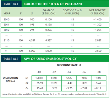
Numerical Example: We can make this concept more concrete with a simple example. Suppose that, absent government intervention, 100 units of a pollutant will be emitted into the atmosphere every year for the next 100 years; the rate at which the stock dissipates, δ, is 2 percent per year, and the stock of pollutant is initially zero. Table 18.1 shows how the stock builds up over time. Note that after 100 years, the stock will reach a level of 4,337 units.
(If this level of emissions continued forever, the stock will eventually approach E/ δ = 100>.02 = 5,000 units). Suppose that the stock of pollutant creates economic damage (in terms of health costs, reduced productivity, etc.) equal to $1 million per unit. Thus, if the total stock of pollutant were, say, 1000 units, the resulting economic damage for that year would be $1 billion. And suppose that the annual cost of reducing emissions is $15 million per unit of reduction. Thus, to reduce emissions from 100 units per year to zero would cost 100 * $15 million = $1.5 billion per year. Would it make sense, in this case, to reduce emissions to zero starting immediately?
To answer this question, we must compare the present value of the annual cost of $1.5 billion with the present value of the annual benefit resulting from a reduced stock of pollutant. Of course, if emissions were reduced to zero starting immediately, the stock of pollutant would likewise be equal to zero over the entire 100 years. Thus, the benefit of the policy would be the savings of social cost associated with a growing stock of pollutant. Table 18.1 shows the annual cost of reducing emissions from 100 units to zero, the annual benefit from averting damage, and the annual net benefit (the annual benefit net of the cost of eliminating emissions). As you would expect, the annual net benefit is negative in the early years because the stock of pollutant is low; the net benefit becomes positive only later, after the stock of pollutant has grown.
To determine whether a policy of zero emissions makes sense, we must calculate the NPV of the policy, which in this case is the present discounted value of the annual net benefits shown in Table 18.1. Denoting the discount rate by R, the NPV is:
NPV = (-1.5 + .1) + (-1.5 + .198) / (1 + R) + (-1.5 + .296) / ((1 + R)^2) + … + (-1.5 + 4.337) / ((1 + R)^99))
Is this NPV positive or negative? The answer depends on the discount rate, R. Table 18.2 shows the NPV as a function of the discount rate. (The middle row of Table 18.2, in which the dissipation rate δ is 2 percent, corresponds to Table 18.1. Table 18.2 also shows NPVs for dissipation rates of 1 percent and 4 percent). For discount rates of 4 percent or less, the NPV is clearly positive, but if the discount rate is large, the NPV will be negative.
Table 18.2 also shows how the NPV of a “zero emissions” policy depends on the dissipation rate, δ. If δ is lower, the accumulated stock of pollutant will reach higher levels and cause more economic damage, so the future benefits of reducing emissions will be greater. Note from Table 18.2 that for any given discount rate, the NPV of eliminating emissions is much larger if δ = .01 and much smaller if δ = .04. As we will see, one of the reasons why there is so much concern over global warming is the fact that the stock of GHGs dissipates very slowly; δ is only about .005.
697
Even if worldwide GhG emissions were to be stabilized at current levels, atmospheric GhG concentrations would continue to grow throughout the next century.
US-6-m
426
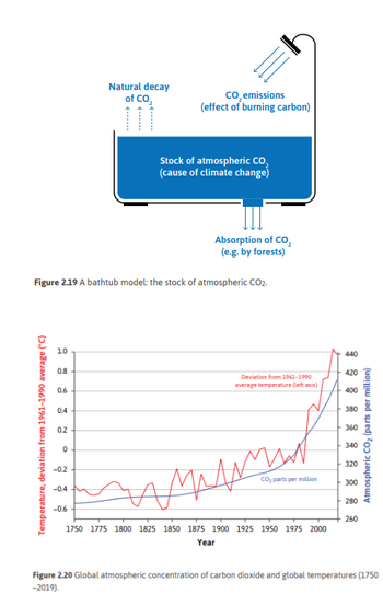
CO2 and other greenhouse gas emissions remain in the atmosphere for a long time, decades or even centuries. This means that even if we reduce annual emissions by 50 percent or more, total concentrations will continue to rise. The atmosphere can be viewed as a bathtub with a very, very slow leak. As long as we keep adding more water (i.e., greenhouse gases) beyond a slight trickle to the bathtub, its level will continue to rise.
427
Cost-benefit analysis of climate change is particularly difficult for two main reasons: the high degree of uncertainty about future impacts and the long period of the analysis.
US-8-m
799
It is largely irreversible, particularly in its effect on rising sea levels and on ecosystems.
802
The difficulty with addressing these effects is that unlike air or water pollution that can be seen today, climate change has a cumulative effect. In other words, this year's CO2 adds to that from the past to raise concentrations in the future. Once CO2 levels reach a certain level, it may lead to extreme consequences that cannot be reversed. The global environment is essentially a common resource with many public goods aspects, and climate change is a huge global negative externality that extends long into the future.

US-16-m
92
The amount of CO2 in the atmosphere is called the stock, while the amount being added per year is called the flow. To better understand what the terms stock and flow mean, consider Figure 2.19. The stock of CO2 is the amount in the bathtub. A flow is a measure based on a time period, like the number of tons of CO2 per year. CO2 emissions are an inflow that adds to the amount of atmospheric greenhouse gases, while the natural decay of CO2 and its absorption (for example, by forests) are outflows that reduce the amount. A key fact of climate science is that global warming results from the stock. It’s what’s in the tub that matters. The flow matters only because it will alter the stock. Figure 2.20 illustrates the movements in the stock of atmospheric CO2 and annual temperatures. The increase in the stock of atmospheric CO2 is occurring because the outflows (natural decay, and absorption by forests and other carbon sinks) are far less than the new emissions that we add annually. Moreover, deforestation in the Amazon, Indonesia, and elsewhere is reducing the CO2 outflows while also adding to CO2 emissions. Forests are often replaced by agriculture, which produces further green house gas emissions—including methane from livestock, and nitrous oxide from fertilizer overuse. The natural decay of CO2 is extraordinarily slow. Of the carbon dioxide that humans have put in the atmosphere since the mass burning of coal that started in the Industrial Revolution, two-thirds will still be there a hundred years from now. More than a third will still be ‘in the tub’ a thousand years from now. The natural processes that stabilized greenhouse gases in pre-industrial times have been entirely overwhelmed by human economic activity. And the imbalance is accelerating.
444
Flow: A quantity measured per unit of time, such as weekly income, or annual carbon emissions.
Stock: A quantity measured at a point in time, such as a firm’s stock of capital goods, or the amount of carbon dioxide in the atmosphere. Its units do not depend on time.
US-8-M
340
A second issue arises in cases in which high levels of current emissions produce irreversible outcomes. Some would argue that by the time nations such as China and Vietnam develop enough to reduce their emissions, it will be too late. Many believe that global warming is such an example.
FR-2-m
300
Par ailleurs, ils font remarquer que les coûts liés à la pollution et les impacts du changement climatique sont sans cesse réévalués à la hausse, avec la mise en avant de risques majeurs (effets de seuil, irréversibilités, etc.).
FR-2-B
153
Cette dernière conception [durabilité] repose sur le constat que certains dégâts sur la nature sont irréversibles et qu'il existe des points de basculement quant aux atteintes à l'environnement. La limite de 2 °C en plus pour les températures mondiales en serait un exemple, le risque étant un emballement incontrôlable des phénomènes naturels si elle est franchie.